Reinforcement Learning

Reinforcement Learning: Definitions
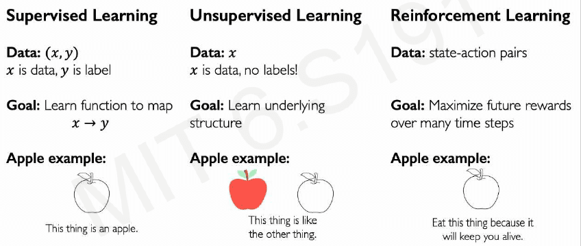
RL is a branch of Machine Learning suitable for learning in dynamic enviroments, such as robotics and gameplay/strategy.
 From MIT online lectures
Let's go over the classical RL definitions:
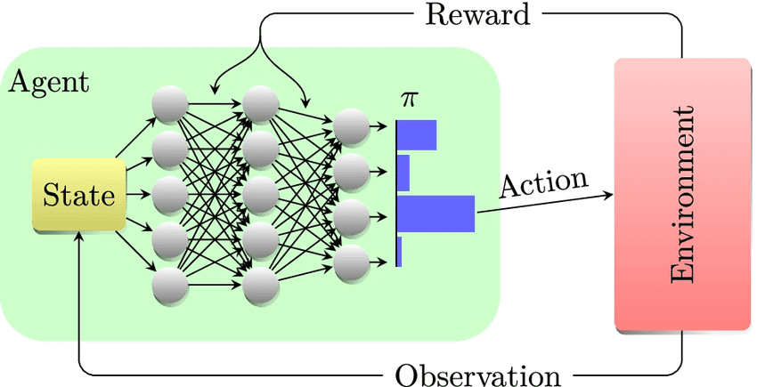
Agent: Entity that takes actions. E.G. Mario in Mario Bros Environment: The world in which the agent exists and operates Action: A command or move that the agent can make in the environment E.G. Move right Action space A: The set of possible actions an agent can make in the environment (← → jump) ; can be continuous Observations: Information the agent receives from the environment at each time step. It’s what the agent perceives, which may be partial in some cases (the agent may be unable to fully observe everything). In the form of:
-
State: A situation which the agent perceived at a given instant in time
-
Reward: Feedback that measures the success or failure of the agent’s action, relative to the goal. E.g: touch a coin and get points in MB
💡 The agent chooses actions to maximize long-term rewards based on what it observes
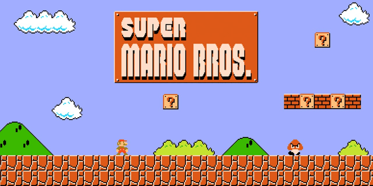
I always love to use Super Mario Bros analogy to remember the definitions:
| Concept | Mario Bros equivalent | |
|---|---|---|
| Agent | Mario (character) |  |
| Environment | The entire map level and all its features | 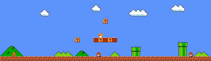 |
| Action Space | move forward, backwards, jump, attack | 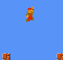 |
| State | Mario's precise x,y position ; enemy positions, velocity, time remaining, etc. mario never sees the whole thing though! it observes a partial, cropped version of it. | |
| Reward | Could be in the lines of: +1 for collecting a coin +100 for defeating an enemy +1000 for finishing a level -1 for dying +0.1 for moving right |  |
At time , the agent is in a state . It will take action . It will get a reward . It will transition to .
The total reward at time t, or return, is , i.e. all future returns added, with an extra discount factor to encourage greedy choices.
 The return is the total future reward you will receive given your policy.
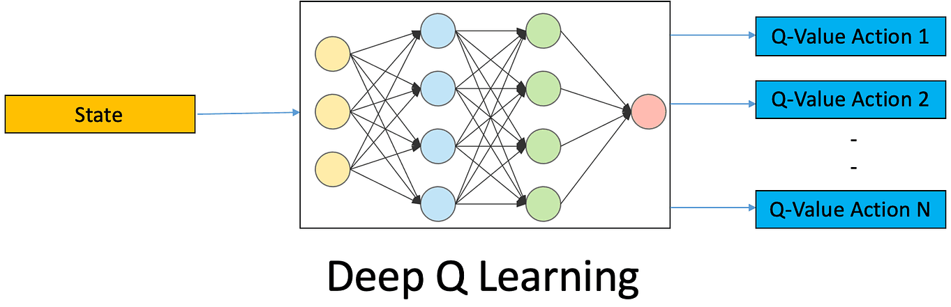
Q-Function: Function that captures the expected total future reward an agent in state can receive by executing action .
Policy : gives us the best action to take at state . This is ultimately what we want to find.
 The policy is basically the function that decides which action to take next
Deep RL
Deep RL is basically how to solve this problem using deep neural networks. We have different options, such as:
Value Learning
Learn a value function Q directly, there is no concept of policy in this approach.
Remember that Q(s,a) = expected return starting from state and taking action , so it basically predicts how good an action is by estimating the total final reward you'll get at the end of the day.
A neural network is used to learn to predict a scalar value (score) given state and action inputs. An implicit policy is derived:
Policy Learning
The policy is learned directly. We learn which action to take, no need to compute Q-values.
At first, policy learning and Q learning may seem identical. You have a NN whose input is the state and whose output gives you a per-action score that defines the next action. The network architectures to solve the problem can probably be identical and work for either approach.
Let's jump back to the Mario bros example though, so we can better understand why these are different approaches. Imagine we are in a specific state .
| Next action | Q | P |
|---|---|---|
| left | Q(s,left) = 0.2 | P(s,left) = 0.1 |
| right | Q(s,right) = 0.4 | P(s,right) = 0.25 |
| jump | Q(s,jump) = 0.9 | P(s,jump) = 0.6 |
| run | Q(s,run) = 0.1 | P(s,run) = 0.05 |
- Q is predicting the total reward of picking each action
- P is predicting a probability distribution over actions, from which we sample the next action
The meaning of the outputs, the training signal and the gradient updates are completely different. A classifier of cats vs dogs has the same shape as a classifier for spam vs not-spam ; but they are not the same problem.
Both approaches usually employ different loss functions, training strategies, etc. Moreover, pi can output the action directly (no need to explicitly calculate the probabilities) - this makes it able to handle continuous action spaces.
Actor-critic methods
A hybrid of policy learning (actor) and value learning (critic).
The actor is a NN that outputs the policy: it takes a state and outputs the policy:
- -> probability of taking each action in a discrete scenario or
- the parameters of a continuous distribution over actions
The critic is another NN that estimates value, usually either:
- V(s): state value or
- Q(s,a): action value
The actor makes decision, the critic tells the action how good decisions were. This is used as follows:
-
Actor picks an action based on
-
Environment returns a reward and
-
Critic computes a score , which tells whether the action was good (positive) or bad (negative)
-
Actor updates its weights (parameters) to increase probability of good actions, based on the feedback it received from the critic:
-
Critic updates
V(s)(its internal parameters) by using MSE on the TD.Temporal Difference (TD) Learning: You learn from the difference between what you expected to happen and what actually happened one time step later.
Training RL models and continuous learning
This is something that I struggled to envision at first, because I am so familiar with supervised learning settings. In supervised learning or in LLMs, you first train and then the deployed model has static weights and stops learning.
Often RL is also seen in this way:
- You train a NN offline in some dataset to learn e.g. the policy or the Q value function.
- You deploy this model, and it never changes its weights again.
- At deployment, it only chooses actions.
Most algorithms though never stop learning.
- The agent learns while acting
- Gradient updates happen after every step (or mini batch of steps)
- The agent creates its own training data by exploring
- That online learning is what allows it to improve its policy
This is a big conceptual jump, and it is also why this rebranded concept of world models is taking center stage.
Supervised learning = learn first, act later.
RL = learn by acting, and keep learning.
Here is another possible training scenario for policy-based NNs:

 The loss is high when you did something wrong.